Variational Inference w/ EM algorithm (Part 2)
Motivation
In the last post of this two-part series, I introduced the theory behind mean-field variational inference. In this post, I’ll walk through my implementation of mean-field VI on the task of polygenic risk score (PRS) regression with spike-and-slab prior.
What is PRS?
To understand polygenic risk score prediction, we first have to introduce the concept of genome-wide association studies (GWAS). In a GWAS, we are given a dataset of \(N\) individuals, each with a set of \(M\) genetic variants (SNPs) and a binary phenotype (e.g. disease status). The goal of GWAS is to identify which SNPs are associated with the phenotype, and to quantify the strength of these associations. In other words, we want to find the SNPs that are statistically significant, and to estimate the effect size \(\beta_i\) of each SNP \(i\) on the phenotype \(y\).
Typically, we use a linear model to fit the data, where the phenotype \(y\) is a linear combination of the SNPs \(x\), with some noise \(\epsilon\):
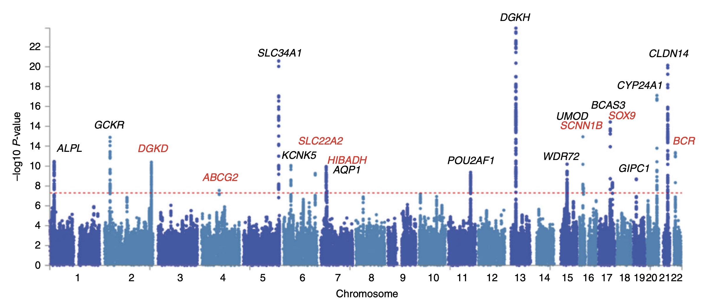
\[y = \beta_0 + \sum_{i=1}^M \beta_i x_i + \epsilon\]We can then use \(\beta_i\) to quantify the strength of the association between SNP \(i\) and the phenotype \(y\). After doing some statistical tests on \(\beta_i\), we typically end up with a list of SNPs that are statistically significant and we can obtain nice Manhattan plots like this:

Naturally, a good follow-up question is: how well can we predict the phenotype \(y\) given the SNPs \(x\)? This is where polygenic risk score (PRS) prediction comes in. The idea is to use the estimated effect sizes \(\beta_i\) to compute a weighted sum of the SNPs \(x\), which we call the polygenic risk score \(s\). These scores can inform us about the genetic risk of an individual developing a disease, and can be used to predict the phenotype \(y\).
However, there are a few issues with this approach. First, the effect sizes \(\beta_i\) are estimated from a linear model, which assumes that the phenotype \(y\) is a linear combination of the SNPs \(x\). This is not always the case, since the phenotype \(y\) is often a non-linear function of the SNPs \(x\), like in epistasis. Second, the linear model assumes independence between the SNPs \(x\), the phenotype \(y\), and the noise \(\epsilon\), which is not necessarily true. These assumptions can lead to poor predictive performance of the PRS.
Given that the effect sizes \(\beta\) predicted by the linear model are noisy as explained above, we can use Bayesian inference to inject our prior domain knowledge into the model. If the prior is meaningful, then the new posterior estimate of \(\beta\) should be more accurate than the original linear estimates, leading to better predictive performance of the PRS.
In this post, we will use mean-field variational inference to estimate the posterior distribution of \(\beta\) with a spike-and-slab prior.
Spike-and-slab prior
Intuitively, given a specific phenotype \(y\), only a very small subset of all the ~20000 genes will be causally related to the it. This means that the true effect sizes of most genes should be zero, and only a handful of genes should have non-zero effect sizes. The spike and slab prior allows us to model this belief by assuming that the effect sizes \(\beta_i\) are either zero or drawn from a normal distribution with zero mean and variance \(\sigma_{\beta}^2\). The probability of a non-zero effect size is given by the spike probability \(\pi\), which is the proportion hyperparameter of a Bernouilli.
\[\begin{equation} \label{eq:prior} \begin{split} s_i & \sim \text{Bernouilli}(\pi) \\ \beta_i & |s_i=1 \sim \mathcal{N}(0, \sigma_{\beta}^2) \\ p(\beta_i, s_i) & = \mathcal{N}(\beta_i \vert 0, \sigma_{\beta}^2)\pi^{s_i}(1-\pi)^{1-s_i} \\\\ \end{split} \end{equation}\]class Bernoulli(Distribution):
p: float
def __init__(self, p) -> None:
super().__init__()
self.p = p
def pdf(self, x):
return self.p**x * (1-self.p)**(1-x)
def logpdf(self, x):
return x*np.log(self.p) + (1-x)*np.log(1-self.p)
def expectation(self):
return self.p
def expectation_log(self):
return self.p * np.log(self.p) + (1-self.p) * np.log(1-self.p)
def update_p(self, p):
self.p = p
Likehood
The likelihood simply models the probability of the phenotype \(y\) given the SNPs \(x\), the effect sizes \(\beta\), and the boolean causal indicators \(s\) as a normal distribution centered at the model output with environmental variance \(\sigma_{\epsilon}^2\), that is not captured by the model.
\[\begin{split} p(y\vert X,\beta, s) = \mathcal{N}(X (s \circ \beta), \sigma_{\epsilon}^2) \\\\ \end{split}\]class Normal(Distribution):
mu: float
sigma: float
def __init__(self, mu, sigma) -> None:
super().__init__()
self.mu = mu
self.sigma = sigma
def pdf(self, x):
return multivariate_normal.pdf(x, mean=self.mu, cov=self.sigma)
def logpdf(self, x):
return multivariate_normal.logpdf(x, mean=self.mu, cov=self.sigma)
def expectation(self):
return self.mu
def update_mu(self, mu) -> None:
self.mu = mu
def update_sigma(self, sigma) -> None:
self.sigma = sigma
Variational distribution
Now, we can derive the variational distribution \(q\) that we will use to approximate the posterior distribution \(p\). Recall from part 1, that to get \(q\), we need to factorize the ELBO objective into a product of independent causal variables \(z_i\) using the mean-field assumption, and then maximize the ELBO with respect to each \(z_i\) to obtain closed form expression for \(q\).
Recall that under the mean-field assumption, we can factorize the ELBO as follows:
\[\begin{equation} \label{eq:elbo} \begin{split} \text{ELBO}(q\vert\phi) & = \sum_j \int q(z_j)\log \frac{\text{exp}(\mathbb{E}_{q(z_i)}[\log p(X,z)]_{i\neq j})}{q(z_j)}dz_j - \sum_{i\neq j}\int q(z_i)\log q(z_i)dz_i \\ & = -\mathbb{KL}[q_j \| \tilde{p}_{i\neq j}] + \mathbb{H}(z_{i\neq j}) + C \\ \end{split} \end{equation}\]Further, recall that this expression is maximized only if \(-\mathbb{KL}[q_j \| \tilde{p}_{i\neq j}] = 0\) for all \(j\), which occurs when \(\log q(z_j\vert\phi) = \log \tilde p_{i\neq j}\). We use this constraint to derive closed form for the variational distribution \(q(\beta,s\vert y,X) = \prod_{j} q(\beta_j\vert s_j)q(s_j)\).
First, let’s derive \(q^*(\beta_j\vert s_j)\) by completing the square:
\[\begin{equation} \begin{split} \log q^*(\beta_j\vert s_j=1) & = \log \tilde p_{i\neq j} \\ & = \frac{1}{C'}\mathbb{E}_{q(\beta_i, s_i)}[\log p(y\vert X,\beta,s)+\log p(\beta_j)]_{i\neq j} \\ & \propto \mathbb{E}_{q(\beta_i, s_i)}\Biggr[-\frac{1}{2}\Biggl\{(\tau_{\epsilon} x^T_jx_j+\tau_\beta)\beta_j^2 - 2\tau_\epsilon(y-\hat{y}_i)^Tx_j\beta_j\Biggl\}\Biggr]_{i\neq j} \\ & \sim \mathcal{N}(\mu^*_{\beta_j}, \frac{1}{\tau^*_{\beta_j}}) \\ & \text{where} \\ & \tau^*_{\beta_j} = \tau_\epsilon x^T_jx_j+\tau_\beta \\ & \mu^*_{\beta_j} = \frac{\tau_\epsilon}{\tau^*_{\beta_j}}\mathbb{E}_{q(\beta_i,s_i)}[(y-\hat{y_i})^Tx_j]_{i\neq j} = N\frac{\tau_\epsilon}{\tau^*_{\beta_j}}\Biggl(\frac{y^Tx_j}{N}-\sum_{i\neq j}\gamma^*_i \mu^*_{\beta_i} r_{ij} \Biggl) \\ \end{split} \end{equation}\]Now, let’s derive \(q^*(s_j)\):
\[\begin{split} \log q(s_j=1) & = \log \tilde p_{i\neq j} \\ & = \frac{1}{C'}\mathbb{E}_{q(s_i)}[\log p(y\vert \hat{y_i},s_j=1)+\log p(s_j=1)]_{i\neq j} \\ & \propto \frac{N}{2}\log\tau_{\epsilon}-C+\frac{1}{2}\log\tau_{\beta}-\frac{1}{2}\tau^*_{\beta_j}+\frac{\tau^*_{\beta_j}}{2}{\mu^*_{\beta_j}}^2+\log{\pi} \\\\ \log q(s_j=0) & \propto \frac{N}{2}\log\tau_{\epsilon}-C+\log{1-\pi} \\\\ q^*(s_j) & = \frac{\text{exp}(\log q(s_j=1))}{\text{exp}(\log q(s_j=0)) + \text{exp}(\log q(s_j=1))} \\ & = \frac{1}{1+\text{exp}(-u_j)} = \gamma^*_j \\ & \text{where}\;\; u_j = \log\frac{\pi}{1-\pi} + \frac{1}{2}\log\frac{\tau_\beta}{\tau^*_{\beta_j}}+\frac{\tau^*_{\beta_j}}{2}{\mu^*_{\beta_j}}^2 \\ \end{split}\]class Variational(Distribution):
m: int
latents: List[Tuple[Normal, Bernoulli]]
def __init__(self, m) -> None:
super().__init__()
self.m: int = m
def setup(self, mu: float, precision: float, gamma: float) -> None:
self.latents = [(Normal(mu, 1/precision), Bernoulli(gamma)) for _ in range(self.m)]
def pdf(self, beta, s):
return np.prod([self.latents[i][0].pdf(beta[i]) * self.latents[i][1].pdf(s[i]) for i in range(self.m)])
def logpdf(self, beta, s):
return np.sum([self.latents[i][0].logpdf(beta[i]) + self.latents[i][1].logpdf(s[i]) for i in range(self.m)])
def update_mu(self, mu, j):
self.latents[j][0].update_mu(mu)
def update_sigma(self, precision, j):
self.latents[j][0].update_sigma(1/precision)
def update_gamma(self, gamma, j):
self.latents[j][1].update_p(gamma)
def get_mu(self):
return np.array([self.latents[i][0].mu for i in range(self.m)])
def get_sigma(self):
return np.array([self.latents[i][0].sigma for i in range(self.m)])
def get_gamma(self):
return np.array([self.latents[i][1].p for i in range(self.m)])
Now that we have found closed form expressions for \(q^*(\beta_j\vert s_j)\) and \(q^*(s_j)\), we can use them to compute the ELBO objective and maximize it with respect to the hyperparameters \(\phi=(\tau_\epsilon,\tau_\beta, \pi)\). However, we will soon realize that we cannot directly solve this optimization problem since there is a circular dependency between the hyperparameters \(\phi\) and the variational distribution parameters \(\tau^*_{\beta_j}, \mu^*_{\beta_j}, \gamma^*_j\). In other words, we need to know the optimal hyperparameters to compute the optimal variational distribution, but we also need to know the optimal variational distribution to compute the optimal hyperparameters. This is where the EM algorithm comes in.
E-step
In the E-step of the EM algorithm, we simply update the variational distribution parameters \(\tau^*_{\beta_j}, \mu^*_{\beta_j}, \gamma^*_j\) using the current fixed hyperparameters \(\phi=(\tau_\epsilon,\tau_\beta, \pi)\). This is done by evaluating the closed form expressions we derived above, i.e.:
\[\begin{equation} \label{eq:estep} \begin{split} & \tau^*_{\beta_j} = \tau_\epsilon x^T_jx_j+\tau_\beta \\ & \mu^*_{\beta_j} = N\frac{\tau_\epsilon}{\tau^*_{\beta_j}}\Biggl(\frac{y^Tx_j}{N}-\sum_{i\neq j}\gamma^*_i \mu^*_{\beta_i} r_{ij} \Biggl) \\ & \gamma^*_j = \frac{1}{1+\text{exp}(-u_j)},\;\; u_j = \log\frac{\pi}{1-\pi} + \frac{1}{2}\log\frac{\tau_\beta}{\tau^*_{\beta_j}}+\frac{\tau^*_{\beta_j}}{2}{\mu^*_{\beta_j}}^2 \\\\ & q(\beta_j\vert s_j=1) = \mathcal{N}(\mu^*_{\beta_j}, \frac{1}{\tau^*_{\beta_j}})\qquad q(s_j=1) = \gamma^*_j \end{split} \end{equation}\]def E_step(self, mbeta: np.ndarray, ld: np.ndarray, n: int) -> None:
"""
Update the latent distribution parameters using the other latents parameters,
the hyperparameters and the observed data.
"""
for j in range(self.var.m):
new_precision = n * ld[j][j] * self.hparams["tau_epsilon"] + self.hparams["tau_beta"]
new_mu = n*self.hparams["tau_epsilon"]/new_precision * \
(mbeta[j] - np.sum(np.delete(np.prod(np.vstack([ \
self.var.get_mu(), self.var.get_gamma(), ld[j]]), axis=0), j)))
new_uj = np.log(self.hparams["pi"] / (1-self.hparams["pi"])) \
+ 0.5 * np.log(self.hparams["tau_beta"] / new_precision) \
+ new_precision/2*(new_mu**2)
new_gamma = 1 / (1 + np.exp(-new_uj))
self.var.update_mu(new_mu, j)
self.var.update_sigma(new_precision, j)
self.var.update_gamma(new_gamma, j)
# After a full cycle of updates, we cap gamma to avoid numerical instability
for j in range(self.var.m):
self.var.update_gamma(np.clip(self.var.latents[j][1].p, 0.01, 0.99), j)
M-step
In the M-step, we use the updated variational distribution to maximize the ELBO objective with respect to the hyperparameters \(\phi=(\tau_\epsilon,\tau_\beta, \pi)\). This is done by setting the gradient of the ELBO objective with respect to each hyperparameter to zero, and solving for the optimal hyperparameters.
\[\begin{split} & \frac{\partial \, \text{ELBO}}{\partial \tau_\epsilon} = 0 \iff \tau_\epsilon^{-1} = \mathbb{E}_q[\frac{1}{N}(y-X(s\circ\beta)^T(y-X(s\circ\beta)))] \\\\ & \frac{\partial \, \text{ELBO}}{\partial \tau_\beta} = 0 \iff \tau_\beta^{-1} = \sum_j \gamma^*_j({\mu^*_j}^2+{\tau^*_{\beta_j}}^-1)/\sum_j\gamma^*_j \\\\ & \frac{\partial \, \text{ELBO}}{\partial \pi} = 0 \iff \pi = \frac{1}{M}\sum_j \gamma^*_j \\ \end{split}\]def M_step(self) -> None:
"""
Update the hyperparameters using the current latent parameter estimates and the data.
In this tutorial, we don't update the tau_epsilon hyperparameter for simplicity.
"""
new_tau_epsilon = self.hparams["tau_epsilon"]
new_tau_beta_inv = np.sum(np.multiply( \
self.var.get_gamma(), np.power(self.var.get_mu(), 2) + self.var.get_sigma())) \
/ np.sum(self.var.get_gamma())
new_pi = 1/self.var.m * np.sum(self.var.get_gamma())
self.hparams["tau_epsilon"] = new_tau_epsilon
self.hparams["tau_beta"] = 1/new_tau_beta_inv
self.hparams["pi"] = new_pi
Algorithm
Now that we have derived the E and M steps, we can simply alternate between them until the ELBO objective converges to a maximum.
def compute_elbo(self, mbeta: np.ndarray, ld: np.ndarray, n: int) -> float:
    """
    Compute the evidence lower bound (ELBO) of the model by using the current variational
    distribution and the joint likelihood of the data and the latent variables. These
    distributions are parameterized by our current estimates of hyperparameter values and
    latent distribution parameters.
    """
    exp_var_s = np.sum([v[1].expectation_log() for v in self.var.latents])
    exp_var_beta = -0.5 * np.log(self.hparams["tau_beta"]) * np.sum(self.var.get_gamma())

    summand = np.multiply(self.var.get_gamma(), \
                              np.power(self.var.get_mu(), 2) + self.var.get_sigma())

    exp_true_beta = -0.5 * self.hparams["tau_beta"] * np.sum(summand)
    exp_true_s = np.sum(self.var.get_gamma() * np.log(self.hparams["pi"])   \
                        + (1 - self.var.get_gamma()) * np.log(1 - self.hparams["pi"]))

    double_summand = 0
    for j in range(self.var.m):
        for k in range(j+1, self.var.m):
            gamma_j = self.var.latents[j][1].expectation()
            mu_j = self.var.latents[j][0].expectation()
            gamma_k = self.var.latents[k][1].expectation()
            mu_k = self.var.latents[k][0].expectation()
            double_summand += gamma_j*mu_j*gamma_k*mu_k*ld[j][k]

    exp_true_y = 0.5*n*np.log(self.hparams["tau_epsilon"])  \
        - 0.5*self.hparams["tau_epsilon"]*n \
        + self.hparams["tau_epsilon"]*np.multiply(self.var.get_gamma(), self.var.get_mu())@(n*mbeta)    \
        - 0.5*n*self.hparams["tau_epsilon"]*np.sum(summand*ld.diagonal())   \
        - self.hparams["tau_epsilon"]*(n*double_summand)

    return exp_true_y + exp_true_beta + exp_true_s - exp_var_beta - exp_var_s

def run(self, mbeta: np.ndarray, ld: np.ndarray, n: int, max_iter: int, tol: float=1e-3) -> List[float]:
    """
    Run the EM algorithm for a given number of iterations or until convergence.
    """
    elbo = []
    for i in range(max_iter):
        self.E_step(mbeta, ld, n)
        self.M_step()
        elbo.append(self.compute_elbo(mbeta, ld, n))
        if i > 0 and abs(elbo[-1] - elbo[-2]) < tol:
            break
    return elbo
Results
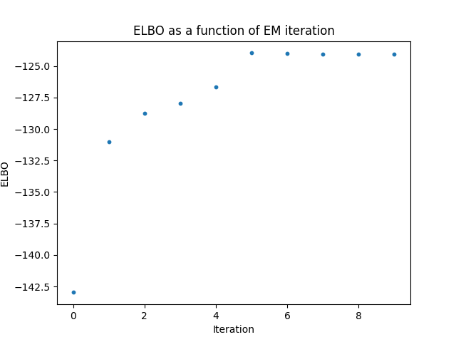
Here are some results I obtained from a simulated dataset with M=100 SNPs given the marginal effect sizes \(\beta\) and the ld matrix \(R\). First let’s take a look at the training curve of the ELBO objective. We can see that the ELBO converges to a maximum after 5 iterations.

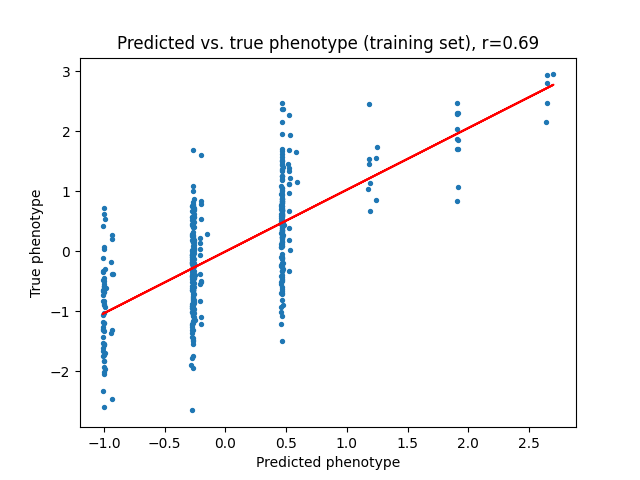
Next, we can take a look at the linear model’s predictions of the phenotype \(y\) given the baseline marginal effect sizes \(\beta\), and compare them to the predictions of the variational model with the new posterior effect sizes \(\beta^{new}\). We can see that the variational model is able to better capture the relationship between the SNPs and the phenotype, which is expected since the variational model is able to incorporate our prior domain knowledge about the SNPs.


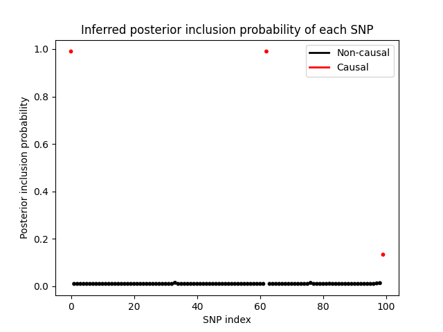
Finally, let’s take a look at posterior inclusion probability of each SNP, which is the probability that the SNP has a non-zero effect size. We can see that the variational distribution \(q(s)\) is able to correctly identify the SNPs with non-zero effect sizes.

The complete code for this project can be found here.