A Gentle Intro to Variational Autoencoders
Motivation
Recently, I’ve been going down the rabbit hole of generative models, and I have been particularly interested in the Variational Autoencoder (VAE)
How to frame generative models
When learning generative models, we assume that the dataset is generated by some unknown underlying source distribution \(p_r\). Our goal is to learn a distribution \(p_g\) that approximates \(p_r\) from which we can sample new realistic data points. Unfortunately, we often don’t have access to \(p_r\), so the best we can do is approximate another distribution \(p_{\hat{r}}\) such that \(p_{\hat{r}}\) maximizes the likelihood of producing the dataset if it were to repeatedly sample independently from it.
Now, there are two main ways that we can go about learning \(p_g \to p_{\hat{r}}\)
- Learn the parameters of \(p_g\) directly through maximum likelihood estimation (MLE) by minimizing the KL divergence \(D_{KL}(p_{\hat{r}} \Vert p_g) = \lmoustache p_{\hat{r}}(x) \frac{p_{\hat{r}}(x)}{p_g(x)}dx\).
- Or, learn a differentiable generative function \(g_\theta\) that maps an existing prior distribution \(Z\) into \(p_g\) such that \(p_g = g_\theta(Z)\).
The issue with the first approach is that the KL divergence loss is extremely unstable when the parameters we want to estimate (in this case the parameters of \(p_{\hat{r}}\)) can belong to an arbitrarily large family of distributions. Indeed, if we examine the KL divergence expression, we see that wherever \(p_{\hat{r}}(x) > 0\), \(p_g(x) > 0\) must also be true, otherwise we end up with an exploding gradient problem during learning as the loss goes to infinity. One way to get around this could be to use a “nicer” loss metric between distributions that is smooth and differentiable everywhere such as the Wasserstein distance.
The better approach, used by GAN and VAE, is the 2nd where we learn a generative function \(g_\theta\) that maps a handpicked prior distribution \(Z\) into the data space. The upside of this approach is that hopefully, if all goes well, the parameters of our prior distribution \(Z\) will be mapped to disentangled high-level features of the data. If we achieve this, then we can easily generate new samples with more control and variety, because we can now sample strategically from $z\sim Z$ (which we handpicked) and then evaluate $g_\theta(z)$.
What is an Autoencoder
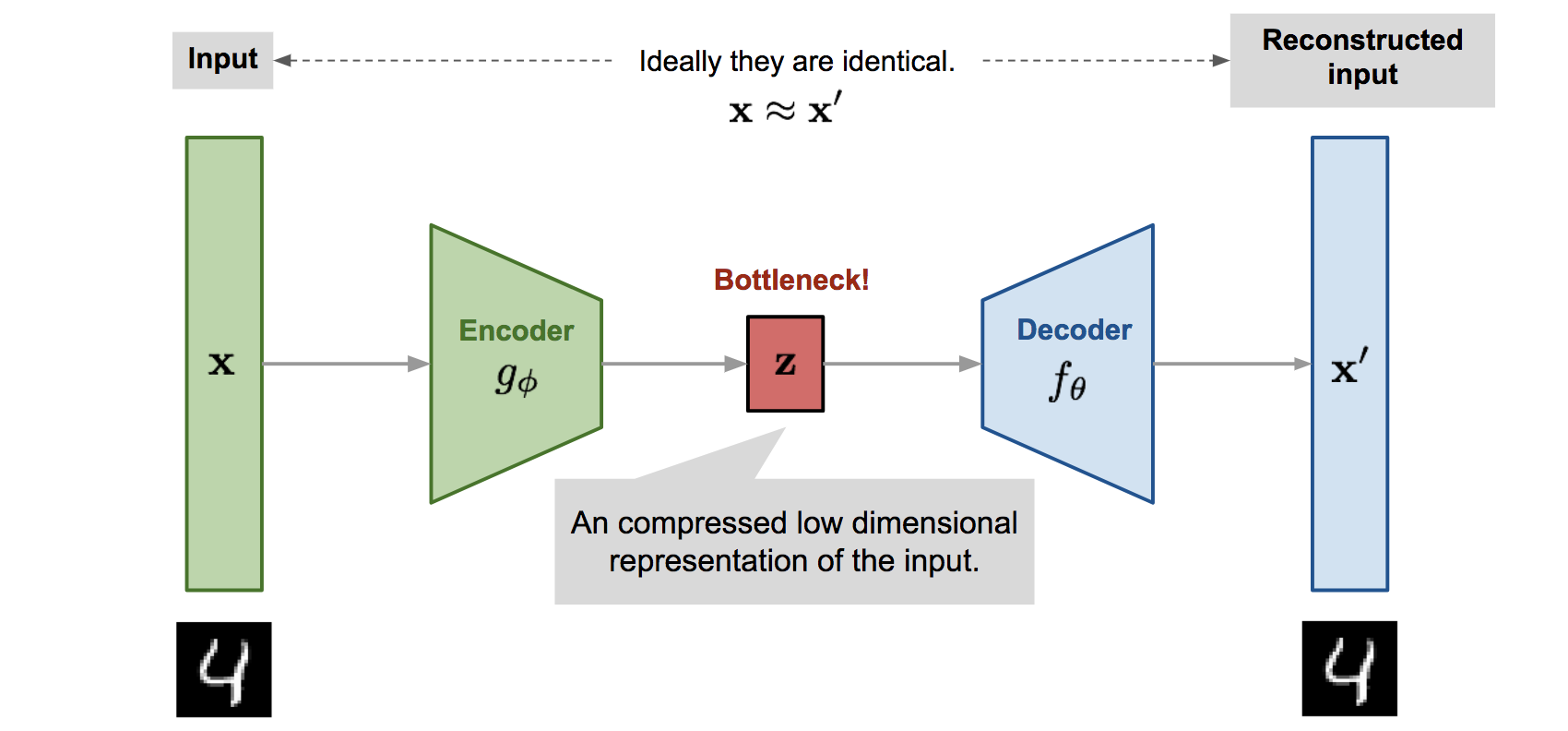
Before I introduce the variational autoencoder, I want to briefly go over its sibling, the autoencoder. The autoencoder is an unsupervised machine learning model whose purpose is to learn a more meaningful representation of the input data in lower dimensional space.
- The encoder learns a function \(f_\phi\) that transforms the high-dimensional input into the low-dimensional latent representation \(z = f_\phi(x)\). Notice here that the latent distribution \(Z\) is unknown and uncontrolled for, meaning that we entirely let the model decide what is the best way to represent the latent embeddings.
- The decoder learns the inverse function \(g_\theta\) that attempts to transform the low-dimensional representation back into the original example such that \(x' = g_\theta(z)\).
- Naturally, the loss function aims to minimize the reconstruction error by minimizing the euclidean distance between the original example and the reconstructed example.
To recap, the goal of the autoencoder is to learn meaningful representations of the data in a lower dimensional latent space by using an encoder-decoder pair.

VAE as a Generative Autoencoder
Recall that fundamentally, a generative model aims to learn a generative function \(g_\theta: Z \to p_g\) mapping the prior distribution \(Z\) into the data space that maximizes the likelihood of generating samples from the dataset. At this point, I hope that it is easier to notice that the function learned by the decoder above does exactly this likelihood maximization since it minimizes the mean squared error loss between the input examples from the dataset and the reconstructed outputs. However as mentioned before, the latent domain of this standard decoder function is uncontrolled for whereas we want our generative function \(g_\theta\) to have a handpicked prior domain \(Z\).
The variational autoencoder (VAE) is thus simply an autoencoder supplemented with an inductive prior that the latent distribution \(Z\) should fit into a pre-selected family of handpicked probability distributions.

How to pick the distribution family for Z
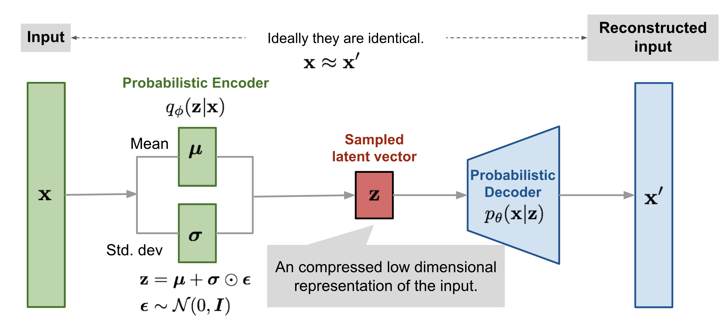
Most often, we constrain the distribution \(Z\) to be a multivariate gaussian distribution with diagonal covariance matrix \(\mathcal{N}(z|\mu, \sigma^2)\). Now that is mouthful, but the real question is why?
Intuitively, we can think of the task of the generative function $g_\theta$ as having to learn something meaningful about the content in the data we wish to generate as well as learning to map the variation in this content to the variation in the low-dimensional latent space \(Z\). As I explained before, we don’t want to \(Z\) to be unconstrained, because we won’t know how to sample cheaply and representatively from it. On the opposite hand, we don’t want to over-constrain \(Z\) either because this might prevent the encoder from learning an expressive and meaningful latent representation of the data. The Gaussian distribution achieves this balance well because it introduces the least amount of prior knowledge into \(Z\) while being extremely easy to sample from.
The diagonal covariance matrix constraint encourages the encoder to learn a multivariate gaussian where each dimension is independent from another. This is desirable when we want to learn the most fundamental sources of variation in the data which often happen to be independent. For example, in the MNIST dataset, we don’t want the model to conflate the representations of the number 1 and 7 just because they share some similarities.
Deriving the VAE loss function
This section of the blog post will be the most math heavy, but I hope that it can provide a better intuition for where the VAE loss comes from. Most resources that I’ve found online directly derive the loss starting from the KL divergence between the estimated and real bayesian posterior distributions of \(z\) conditioned on \(x\), but this seems like it skipped a few steps especially for those who aren’t well-versed in Bayesian theory. Instead, let’s start from first principles.
Recall that our objective is to approximate a distribution \(p_{\hat{r}}\) that maximizes the likelihood of generating the dataset \(D\). To do this, we explicitly defined a prior distribution \(p(z)\) for the latent space and now we are attempting to learn a probabilistic decoder distribution \(p_\theta(x\vert z)\) through our generative function \(g_\theta\). Thus, it should be clear that our goal is to find the parameters \(\theta^*\) such that
\[\begin{split} \theta^* & = \arg \max_{\theta} \mathbb{E}_{x \sim D}[p_\theta(x)] \\ & = \arg \max_{\theta} \mathbb{E}_{x \sim D}[\frac{p_\theta(x|z)p(z)}{p_\theta(z|x)}] \\ \end{split}\]by Bayes Theorem.
First, we note that attempting to learn \(\theta\) directly here using maximum likelihood estimation with loss \(-\log \mathbb{E}_{x \sim D}[p_\theta(x)]\) is impossible because \(p_\theta(x)\), which is known as the evidence in Bayesian statistics, is intractable. If we wanted to compute \(p_\theta(x)\), we would need to marginalize over all values of \(z\) and further, we don’t have access to the posterior distribution \(p_\theta(z\vert x)\).
So we go for a different approach, notice that if we use a neural network to approximate the posterior \(p_\theta(z\vert x)\), then we can manipulate the expectation above to a tractable form. Notably, let \(q_\phi(z\vert x)\) be a probabilistic function learned by the VAE encoder parametrized by \(\phi\) such that our new objective function becomes
\[\begin{split} \theta^* & = \arg \max_{\theta} \mathbb{E}_{x \sim D}[\frac{p_\theta(x|z)p(z)}{q_\phi(z|x)}] \\ & \propto \arg \max_{\theta} \mathbb{E}_{z\sim q_\phi(z|x)}[\log{} p_\theta(x|z)] + \mathbb{E}_{z\sim q_\phi(z|x)}[\frac{p(z)}{q_\phi(z|x)}] \\ & = \arg \min_{\theta} -\mathbb{E}_{z\sim q_\phi(z|x)}[\log{} p_\theta(x|z)] + \mathbb{E}_{z\sim q_\phi(z|x)}[\frac{q_\phi(z|x)}{p(z)}] \\ & = \arg \min_{\theta, \phi} -\mathbb{E}_{z\sim q_\phi(z|x)}[\log{} p_\theta(x|z)] + \mathbb{D_{KL}}(q_\phi(z|x)\Vert p(z)) \\ & = \arg \min_{\theta, \phi} [-\text{likelihood} + \text{KL divergence}] \\ & = \max_{\theta, \phi}ELBO(\theta, \phi) \\ & = \min_{\theta, \phi}L_{VAE}(\theta, \phi) \end{split}\]Notice that this loss expression is exactly what we intuitively wanted to do in the first place. Maximize the likelihood of generating the data from our dataset while adding a regularizer term that encourages the latent space distribution to fit in our gaussian prior \(p(z).\)
Implementing a VAE in PyTorch
Now that we have all the pieces of the puzzle, let’s train a VAE in PyTorch to generate images of characters from the Simpsons. My implementation is based on this great github repository
The dataset
I used a Simpsons dataset of ~20000 character images. Loading the dataset into PyTorch is simply a matter of implementing the torch.utils.data.Dataset class.
class MyDataset(Dataset):
    def __init__(self, data_path: str, split: str, transform: Callable, **kwargs):
        self.data_dir = Path(data_path)
        self.transforms = transform
        imgs = sorted([f for f in self.data_dir.iterdir() if f.suffix == '.jpg'])

        self.imgs = imgs[:int(len(imgs) * 0.75)] if split == "train" else imgs[int(len(imgs) * 0.75):]

    def __len__(self):
        return len(self.imgs)

    def __getitem__(self, idx):
        img = default_loader(self.imgs[idx])

        if self.transforms is not None:
            img = self.transforms(img)

        return img, 0.0 # dummy data label to prevent breaking
The model
We start with the encoder model which takes in a batch of images and outputs the parameters of our multi-variate gaussian distribution \(Z\). In the model architecture declaration below, we use convolutional layers in the encoder body to capture the image features followed by 2 different linear output layers for the mean and variance vectors.
modules = []
in_channels = input_dim
hidden_dims = [32, 64, 128, 256, 512]

# Declare the Encoder Body
for h_dim in hidden_dims:
    modules.append(
        nn.Sequential(
            nn.Conv2d(in_channels, out_channels=h_dim, kernel_size=3, stride=2, padding=1),
            nn.BatchNorm2d(h_dim),
            nn.LeakyReLU()
        )
    )
    in_channels = h_dim

self.encoder = nn.Sequential(*modules)

# Declare the Encoder output layer
self.fc_mu = nn.Linear(hidden_dims[-1]*4, latent_dim)
self.fc_var = nn.Linear(hidden_dims[-1]*4, latent_dim)
Similarly to the encoder, the decoder architecture takes in a latent vector outputted by the encoder, then uses transposed convolution layers to upsample from the low dimensional latent representations. Finally, we use a conv output layer followed by tanh activation function to map the decoder output back to the normalized input pixel space \(\in [-1, 1]\).
# Declare Decoder Architecture
modules = []
hidden_dims.reverse()
self.decoder_input = nn.Linear(latent_dim, hidden_dims[-1]*4)

for i in range(len(hidden_dims)-1):
    modules.append(
        nn.Sequential(
            nn.ConvTranspose2d(hidden_dims[i],
                                hidden_dims[i + 1],
                                kernel_size=3,
                                stride = 2,
                                padding=1,
                                output_padding=1),
            nn.BatchNorm2d(hidden_dims[i + 1]),
            nn.LeakyReLU()
        )
    )

self.decoder = nn.Sequential(*modules)

self.final_layer = nn.Sequential(
    nn.ConvTranspose2d(hidden_dims[-1],
                        hidden_dims[-1],
                        kernel_size=3,
                        stride=2,
                        padding=1,
                        output_padding=1),
    nn.BatchNorm2d(hidden_dims[-1]),
    nn.LeakyReLU(),
    nn.Conv2d(hidden_dims[-1], out_channels=3, kernel_size=3, padding=1),
    nn.Tanh())
Training
During training, we feed the input batch through the encoder to obtain a list of mean and variance vectors. We then sample from this multivariate gaussian using a reparameterization function to obtain a list of latent vectors \([z]\). This step is important because it not only allows us to sample from \(Z\), but also to take a derivative with respect to the encoder parameters during backpropagation. Finally, we feed these latent vectors to the decoder, which outputs a tensor of reconstructed images.
def encode(self, input: Tensor) -> List[Tensor]:
    result = self.encoder(input)
    result = torch.flatten(result, start_dim=1)

    # Split the result into mu and var components
    # of the latent Gaussian distribution
    mu = self.fc_mu(result)
    log_var = self.fc_var(result)

    return [mu, log_var]

def reparameterize(self, mu: Tensor, logvar: Tensor) -> Tensor:
    # Use this to sample from the latent distribution Z
    std = torch.exp(0.5 * logvar)
    eps = torch.randn_like(std)
    return eps * std + mu

def decode(self, z: Tensor) -> Tensor:
    result = self.decoder_input(z)
    result = result.view(-1, 512, 2, 2)
    result = self.decoder(result)
    result = self.final_layer(result)
    return result

def forward(self, input: Tensor, **kwargs) -> Tensor:
    mu, log_var = self.encode(input)
    z = self.reparameterize(mu, log_var)
    return  [self.decode(z), input, mu, log_var]
Finally, we compute the ELBO loss derived above and backpropagate.
def loss_function(self, recons, input, mu, log_var, kld_weight) -> dict:
    # Maximizing the likelihood of the input dataset is equivalent to minimizing
    # the reconstruction loss of the variational autoencoder
    recons_loss =F.mse_loss(recons, input)

    # KL divergence between our prior on Z and the learned latent space by the encoder
    # This measures how far the learned latent distribution deviates from a multivariate gaussian
    kld_loss = torch.mean(-0.5 * torch.sum(1 + log_var - mu ** 2 - log_var.exp(), dim = 1), dim = 0)

    # The final loss is the reconstruction loss (likelihood) + the weighted KL divergence
    # between our prior on Z and the learned latent distribution
    loss = recons_loss + self.beta * kld_weight * kld_loss

    return {
        'loss': loss,
        'Reconstruction_Loss': recons_loss,
        'KLD': kld_loss
    }
Sampling
When we want to sample, we can simply sample a latent vector \(z\) from our multivariate gaussian latent prior \(p(z)\), then feed it through the decoder.
def sample(self, num_samples:int, current_device: int, **kwargs) -> Tensor:
    z = torch.randn(num_samples, self.latent_dim)
    z = z.to(current_device)
    samples = self.decode(z)
    return samples
Results
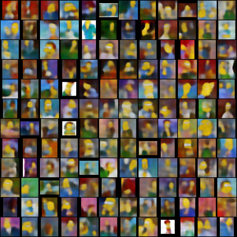
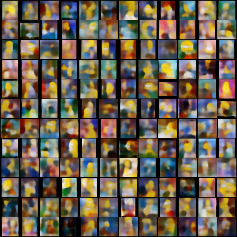
Here are the results of the VAE that I trained on the Simpsons datasets after 100 epochs with 64 batch size. On the left are images recostructed by the model, and on the right are images sampled from the decoder. The results are quite blurry which is a typical symptom of VAEs as the Gaussian prior inductive bias might be acting too strong. Training for more epochs should yield better results.

