Latent Dirichlet Allocation

Motivation

If you’ve ever played around with unsupervised clustering algorithms like k-means, then the concept of topic modeling should already be familiar to you. Informally, topic modelling can be thought of as discovering the underlying “topics” or “themes” that are present in a collection of documents. For example, if we were to apply topic modeling to a collection of news articles, we might expect to find topics like “politics”, “sports”, “entertainment”, etc.

Many topic models are Bayesian probabilistic models that make assumptions about how the dataset documents are generated. We call this the generative process. By performing MLE of the dataset with respect to the model parameters, we can discover the latent variables in the Bayesian model that are responsible for generating the documents. Naturally, different generative processes lead to different topic models. In this post, we’ll be looking at Latent Dirichlet Allocation (LDA) introduced by Blei et al. in 2003.

Generative Process

Given a dataset of $D$ documents, a vocabulary $V$, and a set of $K$ topics, the LDA generative process to create a document $d$ is as follows:

Define a prior distribution over the topic proportions in $d$ from a Dirichlet distribution with parameter $\alpha$:
\[\theta_d \sim \text{Dir}(\alpha)\]
Define a global prior distribution over the word proportions in each topic from a Dirichlet distribution with parameter $\beta$:
\[\phi_k \sim \text{Dir}(\beta)\]
while not done:
1. Sample a topic $z$ from the topic proportions in $d$:
  \[z \sim \text{Multinomial}(\theta_d)\]
2. Sample a word $w$ from the word proportions in $z$:
  \[w \sim \text{Multinomial}(\phi_z)\]
3. Stop with probability $\epsilon$ or continue.

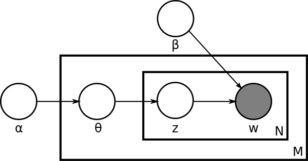
We often use the plate notation to represent the generative process. The plate notation for LDA is shown below:

Plate notation for LDA

Inference

First and foremost, the parameters that we wish to infer in this model are the topic proportions $\theta_d$ and the word proportions $\phi_k$. Notice that these two variables are sufficient to define the entire generative process. In other words, if we know the topic proportions $\theta$ and the word proportions $\phi$ that truly generated the dataset, then we can generate new documents that are indistinguishable from the original dataset. Since we don’t know the true values of $\theta$ and $\phi$, we must infer them from the observed documents $d$ using maximum likelihood estimation of the evidence with respect to these parameters:

\[\begin{align*} \theta^*, \phi^* &= \arg\max_{\theta, \phi} \log p(d | \theta, \phi) \\ &= \arg\max_{\theta, \phi} \log \sum_z p(d, z | \theta, \phi) \\ &= \arg\max_{\theta, \phi} \log \sum_z p(d | z, \theta, \phi) p(z | \theta, \phi) \\ &= \arg\max_{\theta, \phi} \log \sum_z p(d | z, \theta, \phi) p(z | \theta) \\ &= \arg\max_{\theta, \phi} \log \sum_z \prod_{n=1}^N p(w_n | z, \phi) p(z | \theta) \\ &= \arg\max_{\theta, \phi} \log \prod_{n=1}^N \sum_z p(w_n | z, \phi) p(z | \theta) \\ &= \arg\max_{\theta, \phi} \sum_{n=1}^N \log \sum_z p(w_n | z, \phi) p(z | \theta) \end{align*}\]

Unfortunately, this likelihood function is intractable to optimize directly, because we cannot marginalize over all the possible latent topic assignments $z$ for each word $w_n$. Instead, to tackle the partition function $p(d \| \theta, \phi)$, we must turn to approximate inference methods such as variational inference which we introduced in a previous post. Although VI still works here, we will use an approach from the Monte Carlo Markov Chain (MCMC) family of methods called Gibbs sampling.

The idea behind Gibbs sampling is pretty straightforward. In cases where marginalizing the joint distribution $p(z_1, w_1, z_2, w_2, \dots, z_n, w_n \vert \theta, \phi)$ over the latents $z$ is intractable, we can instead sample individual latents from their conditional distributions $p(z_i \vert z_{j\neq i}, x_i, \theta, \phi)$, use these sampled latents to update the parameters $\theta$ and $\phi$ to their new expected values, and repeat this process until convergence.

In the case of LDA, we iteratively sample the latent topic assignments $z_{i,d}$ for each word $w_{i,d}$ in document $d$, and then update the topic proportions $\theta$ and word proportions $\phi$ to their expected values. The conditional distribution for $z_{i,d}$ is given by:

\[\begin{align*} p(z_{i,d} &= k \vert z_{(j,e) \neq (i,d)}, w_{i,d}=v, \theta, \phi) \\ &\propto (\alpha_k + n_{(\cdot,d,k) \neq (v,d,\cdot)})\frac{\beta + n_{(v,\cdot,k) \neq (v,d,\cdot)}}{\sum_w \beta + n_{(w,\cdot,k) \neq (v,d,\cdot)}} \end{align*}\]

Here, $n_{(w,d,k)}$ is the number of times that the word $w \in V$ in document $d$ is assigned to topic $k$. Thus, $n_{(\cdot,d,k) \neq (v,d,\cdot)}$ is the number of words in document $d$ that are assigned to topic $k$, excluding counts of the current word $w_{i,d}=v$. Similarly, $n_{(v,\cdot,k) \neq (v,d,\cdot)}$ is the number of times that word $v$ is assigned to topic $k$ in all documents, excluding the occurrences of $w_{i,d}=v$ in document $d$. Finally, $\sum_w \beta + n_{(w,\cdot,k) \neq (v,d,\cdot)}$ is the total number of words in the vocabulary $V$ that are assigned to topic $k$, excluding the occurrences of $w_{i,d}=v$ in document $d$.

After sampling the topic assignments $z_{i,d}$ for each word $w_{i,d}$ in document $d$, we can update the topic proportions $\theta$ and word proportions $\phi$ to their expected values as follows:

\[\begin{align*} \theta_{d,k} &= \frac{\alpha_k + n_{(\cdot,d,k)}}{\sum_{j=1}^K \alpha_j + n_{(\cdot,d,j)}} \\ \phi_{k,v} &= \frac{\beta + n_{(v,\cdot,k)}}{\sum_{w=1}^V \beta_w + n_{(w,\cdot,k)}} \end{align*}\]

I do not want to claim falsehoods on my blog by deriving these equations myself, so I will refer you to this great resource by Chris Tufts for the full derivation.

Implementation

Now onto the fun part! Let’s implement LDA from scratch in Python. I’ll be using a stripped down version of the MIMIC-III dataset, which is a collection of de-identified medical records from patients admitted to the intensive care unit (ICU). My version contains only the ICD9 codes of timestamped diagnoses for 689 patients with a vocabulary size of 389 unique codes. The dataset is available here

First, we’ll load the dataset and process it into the desired input format for our model which is a list of lists of strings where each sublist represents a document (see patient) and each string represents a word (see ICD code) in the document.

# Format docs into the desired format list of lists
docs = pd.read_csv("data/MIMIC3_DIAGNOSES_ICD_subset.csv.gz", header=0)
docs = docs.sort_values(by=['SUBJECT_ID'])
docs = docs.groupby('SUBJECT_ID')['ICD9_CODE'].apply(list).reset_index(name='ICD9_CODE')
docs = docs['ICD9_CODE'].tolist()

Next, I setup a class to handle manipulations with the latent conditional distribution $p(z_i \vert z_{j\neq i}, x_i, \theta, \phi)$ which we derived above. This class is initialized with the initial parameters $\alpha$ and $\beta$ for the dirichlet priors, the number of topics $K$, and the topic assignment counts matrix $n_{(w,d,k)}$ which is a 3D tensor of shape $V \times D \times K$ where $V$ is the vocabulary size, $D$ is the number of documents, and $K$ is the number of topics.

class LatentDistribution(Distribution):
    alpha: np.ndarray   # 1d array holding alpha hyperparams a_{k}
    beta: float         # beta hyperparam
    n_mat: np.ndarray   # 3d array holding n_{k,d,w}
    K: int              # number of topics

    def __init__(self, K, n_mat, alpha=None, beta=1e-3):
        self.K = K
        self.beta = beta
        self.n_mat = n_mat

        assert n_mat.ndim == 3
        assert n_mat.shape[0] == K

        self.alpha = np.ones(K, dtype=float) if alpha is None else alpha

This class contains methods to sample the conditional distribution $p(z_i \vert z_{j\neq i}, x_i, \theta, \phi)$ and to update the topic proportions $\theta$ and word proportions $\phi$ to their expected values. The sampling method is implemented as follows:

def get_gamma(self, k, d, w):
    alpha_dw = self.alpha[k]
    n_dk = self.n_mat[k,d,:].sum() - self.n_mat[k,d,w]
    n_wk = self.n_mat[k,:,w].sum() - self.n_mat[k,d,w]

    V = self.n_mat.shape[2]
    n_k = self.n_mat[k,:,:].sum() - self.n_mat[k,d,w]
    
    return (alpha_dw + n_dk)*(self.beta + n_wk)/(self.beta*V + n_k)

def pmf(self, d, w):
    g_k = np.array([self.get_gamma(k,d,w) for k in range(self.K)])
    return g_k/g_k.sum()
    
def pdf(self, k, d, w): 
    return self.pmf(d,w)[k]

def sample(self, d, w):
    pmf = self.pmf(d,w)
    return np.random.multinomial(1, pmf).argmax()

The update method is implemented as follows. We also have helper methods to get the current expected values of $\theta$ and $\phi$.

def update_n(self, k, d, w):
    self.n_mat[k,d,w] += 1

def get_phi(self, k, w):
    V = self.n_mat.shape[2]
    n_k = self.n_mat[k,:,:].sum()
    return (self.beta + self.n_mat[k,:,w].sum())/(self.beta*V + n_k)

def get_theta(self, k, d):
    n_d = self.n_mat[:,d,:].sum()
    return (self.alpha[k] + self.n_mat[k,d,:].sum())/(self.alpha.sum() + n_d)

Finally, we are ready to implement the iterative Gibbs inference algorithm. In the class init, we initialize the topic assignment counts matrix $n_{(w,d,k)}$ to zeros, and instantiate a LatentDistribution instance with the correct initial parameters. We also create a vocabulary object which maps each string word to a unique integer index.

class LDA():
    k: int                              # number of topics
    d: int                              # number of documents
    w: int                              # number of words in vocabulary
    vocab: defaultdict                  # vocabulary mapping words to indices
    r_vocab: defaultdict                # reverse vocabulary mapping indices to words
    docs: np.ndarray                    # 2d list holding documents with raw words
    n_iter: int                         # number of iterations
    latent_dist: LatentDistribution     # latent distribution Z

    def __init__(self, k, docs, n_iter=100, alpha=None, beta=1e-3):
        self.k = k
        self.d = len(docs)
        self.docs = docs
        self.vocab = self.setup_vocab(docs)
        self.r_vocab = dict(map(reversed, self.vocab.items()))
        self.w = len(self.vocab)
        self.n_iter = n_iter

        self.n_mat = np.zeros((self.k,self.d,self.w), dtype=int)
        self.latent_dist = LatentDistribution(k, self.n_mat, alpha, beta)

    def setup_vocab(self, docs):
        vocab = defaultdict(int)
        for doc in docs:
            for word in doc:
                if word not in vocab:
                    vocab[word] = len(vocab)
        return vocab

In the fitting method, as explained above, we iterate over each word in each document and sample a new topic assignment $z_{i,d}$ for that word from the conditional distribution. We then update the topic proportions $\theta$ and word proportions $\phi$ to their expected values. We repeat this process for the specified number of iterations.

def fit(self):
    for _ in tqdm(range(self.n_iter)):
        for d in range(self.d):
            for n in range(len(self.docs[d])):
                w = self.vocab[self.docs[d][n]]
                k = self.latent_dist.sample(d,w)
                self.latent_dist.update_n(k,d,w)

Results

Now that we have implemented the LDA model, let’s see what topics it discovers in the MIMIC-III dataset. Given the final topic proportions $\theta$ and word proportions $\phi$, we can get easily get the top words for each topic and the top documents for each topic by sorting the rows and columns of $\phi$ and $\theta$ respectively. We can also correlate the topics with certain sets of keywords to see if the learned topics take on the meaning that we expect. In my dataset, I correlate the topics with 3 key ICD9 categories: Alzheimer’s disease, Parkinson disease, and Multiple Sclerosis. The results are linked below:

Conclusion

In the next post on topic models, I will tackle the older brother of LDA, the embedded topic model (ETM) which is a neural network based topic model that learns the topic proportions $\theta$ and word proportions $\phi$ in an end-to-end fashion in a shared word-topic latent space. Stay tuned!